The Aizawa Attractor
Articles —> The Aizawa Attractor
The Aizawa attractor is a system of equations that, when applied iteratively on three-dimensional coordinates, evolves in such a way as to have the resulting coordinates map out a three dimensional shape, in this case a sphere with a tube-like structure penetrating one of it's axis. The equations themselves are fairly straightforward:
dx = (z-b) * x - d*y
dy = d * x + (z-b) * y
dz = c + a*z - z3 /3 - x2 + f * z * x3
where a = 0.95, b = 0.7, c = 0.6, d = 3.5, e = 0.25, f = 0.1. Each previous coordinate is input into the equations, the resulting value multiplied by a time value (here arbitrarily chosen as 0.01) and then added to the previous value. To place this in the context of a program, and utilizing a previous java class structure developed for the Lorenz Attractor, a new Transform implementation would be of the form:
double dt = 0.01;

double a = 0.95, b = 0.7, c = 0.6, d = 3.5, e = 0.25, f = 0.1;

...

Transform<Tuple3d> aizawa = new Transform<Tuple3d>(){

	@Override

	public Tuple3d transform(Tuple3d val) {

		double x = val.x, y = val.y, z = val.z;

		double x1 = (val.z-b)*val.x - d*val.y;

		double y1 = d * val.x + (val.z - b) * val.y;;

		double z1 = c + a*val.z - (Math.pow(val.z, 3)/3d) -

			(Math.pow(val.x, 2) + Math.pow(val.y, 2)) *

			(1 + e * val.z) + f * val.z * ( Math.pow(val.x, 3));


		Tuple3d t = new Tuple3d(x + dt * x1, y + dt * y1, z + dt * z1);

		return t;

	}

};
In action, the attractor evolves into a beautiful sphere with a tube-like structure penetrating down its y-axis. The image below is the attractor with each generated coordinate colored as a cyan pixel, the initial 'seed' coordinate starting at x = 0.1, y = 0, and z = 0.
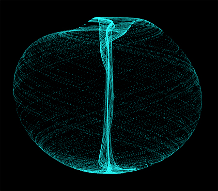
The Aizawa Attractor.
While a static image gives a beautiful rendition of the attractor, putting the attractor in motion can give an even greater depiction of its behavior. In the video below, I rendered the attractor in three dimensions (JOGL/OpenGL) from several different angles and stages.
The Aizawa Attractor. Programmed in Java and rendered using JOGL/OpenGL. Music by Chris Zabriskie, Creative Commons (unaltered).
Initially, several random coordinates were generated and their paths then followed based upon the Aizawa system (their paths defined by a spline curve between subsequent values). Subsequent views show several thousand random points along a single spline trajectory of the attractor.
Notes on Video Construction
Construction of the video went through several trials and modifications. In the initial stages, random coordinates were chosen based upon a uniform distribution between -n and n (on all axis, where n ranged in values under ten). However several points consistently coalesced along the negative z-axis, an unwanted behavior which is seen as a vertical line in the center of the following image:
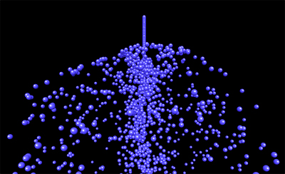
Artifact in the creation of the Aizawa Attractor animation.
To alter this behavior, I decided to analyze how these values evolved. First, one hundred values representing this population were identified by analyzing a frame in which they were at their worst: all coordinates in this frame were sorted based upon their z value and the first one hundred values of the sorted list investigated further. Assuming how these values evolved would be based upon their original value, the coordinates from which they originated (in the first frame) were plotted in R using the pairs function to look for trends.
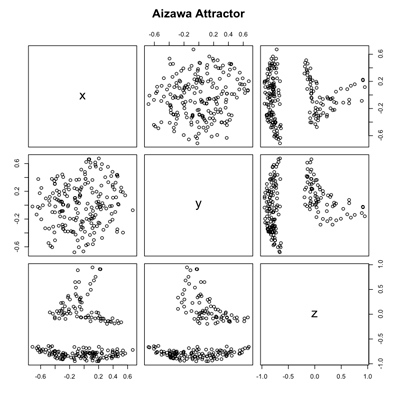
Plot showing the points within the attractor artifact, showing relatively large negative z-axis values contributing to the artifact.
The plot suggests that this concentration of values along the negative z-axis arise from a population of coordinates with larger negative z start values. Thus, to alleviate this artifact the random points generated in the video were offset along the z-axis in the positive direction, allowing for a more uniform and elegant distribution of points as the attractor evolves.
Comments
- Arash Mohammadi - November, 24, 2017
This is one of my favorite attractors. I have just rendered it as a video: https://www.youtube.com/watch?v=RBqbQUu-p00
- Felix Woitzel - December, 26, 2017
I have just copied the formula over to my WebGL particle accelerator and I was confused about the e parameter that you defined but apparently not used then? https://twitter.com/Flexi23/status/945769640797573121
- Jay Mireles James - March, 6, 2018
Hey, this is great! Can you provide a reference for this systems of equations? Where did you come across them? I have not yet been able to locate them in professor Aizawa's papers. Thanks for any information.
- Jay Mireles James - March, 21, 2022
After some time I think I can post the answer to my own question, which is that the system should actually be called ``the Langford system\'\' as it first appeared in \r\n\r\nW. F. Langford. Numerical studies of torus bifurcations. In Numerical methods for bifurcation problems\r\n(Dortmund, 1983), volume 70 of Internat. Schriftenreihe Numer. Math., pages 285–295. Birkh¨auser,\r\nBasel, 1984.\r\n\r\nTakahito Mitsui pointed this out to me in an email some time ago. The literature sourounding the system is discussed more in this paper with Emmanuel Fleurantin:\r\n\r\nhttps://arxiv.org/pdf/1905.08828.pdf