Maze Generation Algorithm - Depth First Search
Articles —> Maze Generation Algorithm - Depth First Search
There are several maze generation algorithms that can be used to randomly generate n-dimensional mazes. In this tutorial I discuss one particular maze generation algorithm that treats a completed maze as a tree, the branches of the tree representing paths through the maze. To generate the tree, a random depth-first search is used - an algorithm which builds the tree randomly until the tree, or maze, is complete. To understand this type of maze generation algorithm in more detail, it helps to understand how the maze is represented as a tree, followed by how the traversal algorithm can be used to generate the maze.
In two dimensions, a maze is a series of paths separated by walls, and to simplify the generation one can think of the maze as a 2-dimensional grid. The grid has a width and height, and each x/y position in the grid can be represented as a cell. When considered in this manner, the grid can be considered a graph G, in which each cell is a node connected to each of its four neighbors by a wall (the exception to this rule is for edge and corner cells which have 3 and 2 neighbors, respectively). The algorithm then finds, based upon a random seed, a spanning tree - or tree composed of all vertices but only some of the edges - of this graph G. The algorithm does so as follows:
- Randomly select a node (or cell) N.
- Push the node N onto a queue Q.
- Mark the cell N as visited.
- Randomly select an adjacent cell A of node N that has not been visited. If all the neighbors of N have been visited:
- Continue to pop items off the queue Q until a node is encountered with at least one non-visited neighbor - assign this node to N and go to step 4.
- If no nodes exist: stop.
- Break the wall between N and A.
- Assign the value A to N.
- Go to step 2.
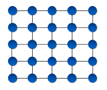
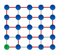
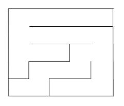
The graph and resulting tree can be visualized more readily by running the algorithm on a small, 5x5 grid of cells as demonstrated in the images and video below. A) The initial graph G where each cell - or node - (depicted as a blue circle) is connected to its neighbors by an edge (depicted as a black line). B) The resulting tree in which the initial node is depicted in green, and the branches depicted in red. C) The branches of the tree represent the paths through the grid, thus the walls between each cell (node) within the tree are removed when two neighboring cells are connected by an edge within the tree, resulting in the final maze. The step-by-step process of generating this maze is illustrated in the video below.
 (A) |
 (B) |
(C)
(A) A 2D grid represented as a graph, (B) the resulting random sparse tree resulting from running the algorithm described above (C) the resulting maze after the maze generation algorithm (green represents the start - or root - node).
Step-by-step generation of the tree above. Green represents the start node, red the end node (see below), and blue the current node.
The above algorithm guarantees a path between the nodes of the resulting spanning tree, thus one can generate start and end points such that the maze - to go from start to end - can be solved. A method to determine start and end points is to constrain the initial random selection in step (1) to an edge cell - a cell along the edges of the grid. To calculate the end, one can mark each edge cell as they are subsequently discovered - the size of the queue Q at that stage is an indication of both distance and difficulty. Thus choosing the most distance cell may seemingly produce the most difficult maze (sometimes this may not always be the case, as visual patterns and tree balance may also play a role in difficulty).
While the above is a simplistic representation of the algorithm, the maze can be made more complex by one or more changes to its structure, for instance increasing its size, transforming the maze coordinates, adding extra dimensions, or rendering the maze in 3D.
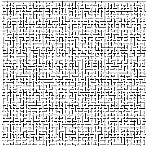
Maze constructed with a 100x100 grid. Both entry and exit on the right.
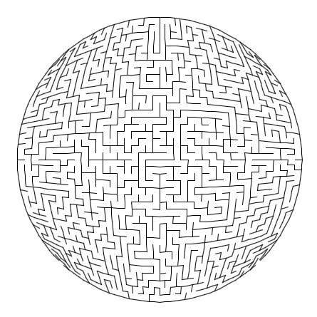
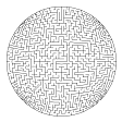
An oval maze. A 40x40 grid was constructed, with each wall (line) being transformed from the grid coordinate to spherical coordinates. See Mapping a Square to a Circle
There are no comments on this article.