Reaction Diffusion: The Gray-Scott Algorithm
Articles —> Reaction Diffusion: The Gray-Scott Algorithm
A Reaction diffusion model is a mathematical model which calculates the concentration of two substances at a given time based upon the substances diffusion, feed rate, removal rate, and a reaction between the two. This simulation not only models the underlying process of a chemical reaction, but can also result in patterns of the substances which are remarkably similar to patterns found in the real world. Examples include patterns on animals1, patterns of veins on a leaf2, and many other biological phenomena3.
To illustrate the model, imagine an area or space containing various concentrations of each substance at time zero. Over time, substance A is fed into the reaction at a given rate, while substance B is removed at a given rate. Further, two molecules of B can react with one of A, which converts the molecule of A to B.
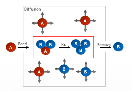
Illustration of the reaction diffusion model. Compound A is fed at a certain rate, while compound B is removed ('killed') at a certain rate. Both compound A and B diffuse at certain rates, and A reacts with 2xB and is converted into compound B.
The simulation is accomplished using two equations, each representing the change in concentration of a substance over time:
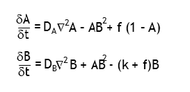
Differential equations defining the change in concentrations of A and B over time. Here f is the feed rate of A, k is the removal/kill rate of B, dA and dB are the diffusion rates of A and B, respectively. These values are adjusted based upon the surrounding concentrations of A or B using a Laplacian Operator (∇2).
The equations may look daunting, but are mathematically quite simple. The change in A (upper equation) is dependent upon its reaction with B (hence - AB2) and is fed at a certain rate (+ f, scaled to its current concentration). The change in B (lower equation) is dependent upon its reaction with A (hence + AB2), and is removed at a given rate ( - k, scaled by the feed rate and concentration of B). The concentration of A or B at each position is updated at each time increment (typically 1) based upon the result of the corresponding equation. The values for the feed rate, removal rate, and diffusion rate are plugged into the equations. The Laplacian Operator ∇2 is a bit more tricky, and relies on a 3x3 convolution matrix. In the simulations below the matrix used was:
| 0.05 | 0.2 | 0.05 |
| 0.2 | -1 | 0.2 |
| 0.05 | 0.2 | 0.05 |
3 x 3 Laplacian convolution matrix.
To calculate the new concentration, the current concentration and each surrounding concentration is multiplied by the corresponding value in the matrix (where the current position corresponds to the center position in the convolution matrix) and all values summed (this value technically represents the difference in concentrations between the current position and the surrounding positions).
The above model was programmed in java (source code available upon request) in which an image represents the reaction 'container' - each pixel of this image represents the concentration of B ([B]) at that position. The concentration of B was updated iteratively, and at each step the pixel values updated: to generate the value of the pixel, [B] was first normalized to global maximum and minimum of [B] followed by some image pixel math to generate the red/green/blue color at that pixel (for an 8 bit image each RGB value ranges from 0-255, to generate darker values for higher [B] the pixel value is calculated using: 255 - [B] * 255). The simulation was ran for various values of the feed, removal, and diffusion rates. Initially, A was seeded at 1.0 and B at zero for every position. Then B was seeded in at pre-defined locations or randomly.
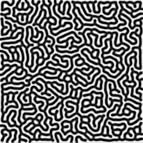
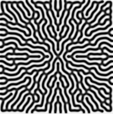
It is interesting to watch the structures unfold while varying the feed rates, removal rate, and diffusion rates - all of which can have dramatic consequences on the process. For instance a feed rate of 0.0367 and a removal rate of 0.0649 results in pockets of high concentrations of B dividing, very similar to the process of cellular division, also known as mitosis. Alternatively, a feed rate of 0.0545 and removal rate of 0.062 results in patterns reminiscent of a fingerprint.
Of course this was a very basic implementation of the model. It can be made more complex by applying feed, removal, and diffusion rates that vary based upon position, as well as implementing color in the resulting image. Further, it would be interesting to implement this in higher dimensions, for instance in 3D where an algorithm such as marching cubes can be used to create the convex hull of the shapes, allowing one to render the shapes using Open GL. This is described in detail in my Reaction Diffusion 3D article.
References
- 1Jonathan B. L. Bard, A Model for Generating Aspects of Zebra and Other Mammailian Coat Patterns, Journal of Theoretical Biology 93 (2) (November 1981) 363-385.
- 2Hans Meinhardt, Models of Biological Pattern Formation, Academic Press, 1982.
- 3A. M. Turing, The chemical basis of morphogenesis, Philosophical Transactions of the Royal Society of London, series B (Biological Sciences), 237 No 641 (1952) 37-72.
- Karl Sims' Reaction Diffusion Tutorial
Comments
- huzaif rahim - April, 14, 2019
How can I get the source code for Reaction Diffusion: the Gray-Scott algorithm,
- Shi Yan - November, 12, 2019
I don't understand why the reaction between A and B is AB^2 ?